Wednesday, December 29, 2010

Rasch Model Origin

Next      Back     Start                            Chapter 9

The Rasch model came into being in response to data that Dr. Georg Rasch graphed. He administered two tests to each student in several grades. The 6th graders made fewer wrong marks than the 5th and 4th graders on the same questions. 


He plotted one test on the horizontal axis and the other on the vertical axis. He observed, “the three assemblies of points which illustrated the amount of errors in the different grades immediately succeeded each other and pointed towards the 0-point.”

Further, he noted that one error on one test (“S”) corresponded to 1.2 errors on the other test (“T5”). This ratio remained the same for each of the three grades, 4th, 5th, and 6th. “An expression for the degree of difficulty of one test in relation to another has thus been found”.

For this constant ratio to happen, the chance to mark a right answer must be equally good whenever the ratio of student proficiency to question difficulty is the same. A student has a 50% chance of correctly marking items when student ability equals question difficulty. “The chances of solving an item thus come to depend only on the ratio between proficiency and degree of difficulty, and this turns out to be the crux of the matter.”

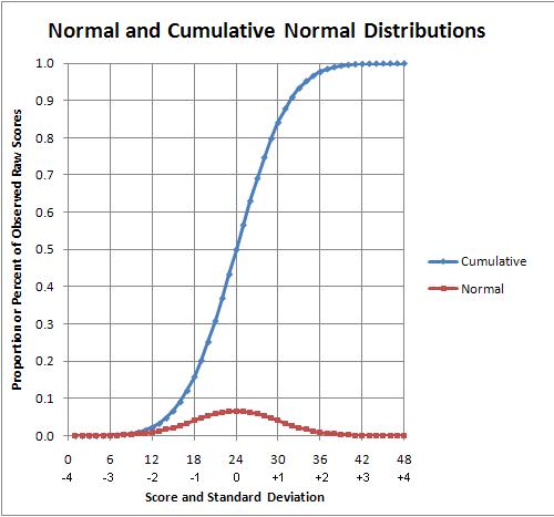
The average wrong score for each of the six tests is marked on the wrong answer ogive (curve). The 5th grade “T5” simulated (5-T5) test had an average score of 50%. This 50% score is located at the zero (0) point on the logit scale. (Remember, an ogive is a normal distribution expressed in logits.)

Applying the Rasch model to the logit values, without further information, only returns the original right mark raw scores: A count of 27 out of 36 total questions is 27/36 or 75%, is odds of right/wrong or 75/25 or 3, and as logits is log(odds) or log(3) or 1.1. In reverse, percent is exp(logits)/(1+exp(logits)) or exp(1.1)/(1+exp(1.1)) or 3/(1+3) or 3/4 or 75%, and is 0.75 of 36 total or a count of 27

The missing information is obtained by replacing the values for marks, 1 and 0, for right and wrong, in a mark data matrix, as in PUP Table 3, with the probability of students making a right mark, that ranges from 0 to 1.

Winsteps fits mark data to the Rasch model, using probabilities, to produce estimated student ability and item difficulty measures on the same horizontal logit scale. It is from these estimated measures that the Rasch model creates (maps) predicted raw scores used as cut scores.

Next     Back     Start

Thursday, December 23, 2010

Perfect Rasch Model

Next    Back    Start                         Chapter 8

Defining relationships creates mathematical models. The sum is the total of all the numbers added. The mean or average is the sum divided by the number of numbers added. The variation in the added numbers is the sum of the squares of the difference between each number and the mean. The mean square or variance is the sum of squares divided by the number of numbers added. The standard deviation (SD) for the mean is the square root of the mean square. These all assume the data fit the normal curve distribution. They are used by both PUP and Ministep.

The cumulative normal distribution (the s-shaped curve or [ogive]) sums the normal distribution. This changes the view of the data from counts by student scores to proportion or percent by student z-scores

Information Response Theory (IRT) is expressed in three models. 
The two-parameter IRT (2-P) model and the cumulative normal distribution almost match. The one-parameter IRT (1-P) model drops out a constant (1.7) needed to make the above match. This gives the 1-P and Rasch model ogives a fixed slope. The three-parameter IRT (3-P) includes guessing. The lower asymptote descends to the test designed guessing value (0.25 for 4-option questions) rather than to zero.

The Rasch model is the easiest model to use with the least requirements. It only requires student scores and item difficulties. It omits discrimination (or slope in 2- and 3-P models) by only using data that fit the perfect Rasch model requirements.

The Rasch model also omits any adjustment for guessing on multiple-choice tests. “Critics of the Rasch model claim this to be a fatal weakness.” (p64, Bond and Fox, 2007). This depends upon how the Rasch model is used. If the area of action is far enough from the lower asymptote, guessing can be of little effect (average score of 75% and cut score of 60%, for example). [Winsteps can clip the lower asymptote.

The all-positive normal scale (0 to 100%) is replaced with a logit scale (-4 to +4). All the ogives, except for the 3-P IRT, cross a point defined as zero logit and 0.5 probability. Student ability and question difficulty are both plotted on the logit scale. A student is expected to mark a right answer 50% of the time when ability and difficulty match. A student with an ability one logit higher than a question with zero logit difficulty is expected to make a right mark 73% of the time.

Item ogives are called item characteristic curves (ICC). A test ogive is called a test characteristic curve (TCC). A TCC is created by combining ICCs. Expected raw scores for setting test cut-scores are obtained by mapping with a TCC from the logit scale.

Next     Back    Start 

Wednesday, December 15, 2010

Standard Units

Next   Back   Start                        Chapter 7

Education has a number of standard units. One is basic to assigning probabilities to events like right marks on a test: the standard deviation.

Random error creates the normal distribution (the normal or bell curve). The distribution happens every time, with a large enough sample. Random error gives each individual an honest and fair chance within the distribution.

The point on the side of the normal curve where it changes bending from up to down, or down to up, is one standard deviation (SD). Some 95% of a sample is expected to fall within +/- 2 SD of the mean. When observed results do not fit within +/- 2 SD (the 5% level of significance) we know to look for a cause, other than chance.

Raw test scores are standardized, turned into Z scores, by dividing them by their SD. Two class distributions can be equated by matching the Z scores or by shifting and stretching one of the distributions to fit the other one. The idea is that students who have similar Z scores should have similar grades. The conversion can be made from Test A to Test B or from Test B to Text A.

Z scores permit adjusting two sets of raw test scores along one dimension. The Rasch model makes adjustments in two dimensions at the same time, raw scores and item difficulty. The Rasch model uses a t-statistic to detect unacceptable fit.

The t Outfit Zstd Outfit Zstd on the Winsteps bubble chart is a standardized indicator of how well student and item performances fit the Rasch model's requirements.

Positive values reflect underfit to the Rasch model or unfinished on PUP Table 3a. Negative values reflect overfit to the Rasch model or highly discriminating on PUP Table 3a. A student or item performance does not fit if the difference is more than two t-statistic units away from the perfect model. Or, for example, the performance of Item 21, 2.3 t Outfit Zstd exceeds two t-statistic units, may still be do to chance one out of 20 times (the 5% [level of significance).

Next    Back   Start

Friday, December 10, 2010

Winsteps Person & Item Bubble Chart

Next    Back    Start                        Chapter 6

Ministep prints out a bubble chart relating how well the estimated measures for persons (blue) and items (red) fit the Rasch model.

A comparison of the two methods for expressing item discrimination (Rasch fitness and PUP item discrimination) reveals an interesting similarity: The two distributions are related. Four of the more difficult items (4, 10, 19, and 21) on the bubble chart show an almost perfect match, on the scatter chart, between fitness and item discrimination.

The Rasch overfit item 4 falls in the PUP distribution at high discrimination (upper left). The Rasch underfit item 21 falls in the PUP distribution at low discrimination (lower right). Fitness and item discrimination are negatively related. The standard fit statistic, outfit,  from Tables 17.1, Person in Measure Order (blue), and 13.1, Item in Measure Order (red) are used in these two charts.

The Rasch model requires uniform discrimination (which is why the model can ignore discrimination after discarding overfit and underfit persons and items, that is, performances that show too high and too low discrimination). Values below -2 are excessive overfit and above +2 are excessive underfit. The person and item performances on this test fit the Rasch model requirements with the exception of item 21. More high scoring students marked it wrong than low scoring students.

The Rasch bubble chart presents results in terms of estimated measures of student ability and item difficulty. The two students (blue) with scores of 100% (high ability) fall at the top of the chart. The three items (red) marked correctly by all students fall at the bottom of the chart (low difficulty).

The three low scoring students (blue 16, 18, and 21) are expected to have less ability (lower on the bubble chart) than needed to answer the two items (red 10 and 19), with an estimated difficulty measure higher (higher on the bubble chart) than their estimated student ability measures.

The bubble chart clearly shows these relationships between students and items. Item fitness on the bubble chart and item discrimination on PUP Table 3a perform similar functions.

Next      Back     Start