Defining relationships creates mathematical models. The sum is the total of all the numbers added. The mean or average is the sum divided by the number of numbers added. The variation in the added numbers is the sum of the squares of the difference between each number and the mean. The mean square or variance is the sum of squares divided by the number of numbers added. The standard deviation (SD) for the mean is the square root of the mean square. These all assume the data fit the normal curve distribution. They are used by both PUP and Ministep.
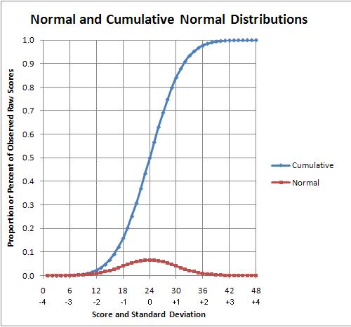
The cumulative normal distribution (the s-shaped curve or [ogive]) sums the normal distribution. This changes the view of the data from counts by student scores to proportion or percent by student z-scores.
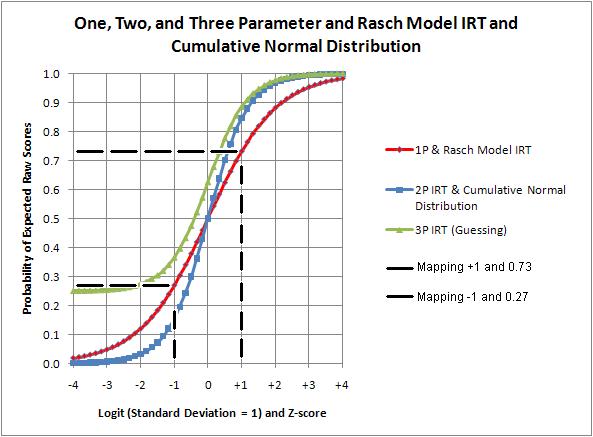
Information Response Theory (IRT) is expressed in three models.
 The two-parameter IRT (2-P) model and the cumulative normal distribution almost match. The one-parameter IRT (1-P) model drops out a constant (1.7) needed to make the above match. This gives the 1-P and Rasch model ogives a fixed slope. The three-parameter IRT (3-P) includes guessing. The lower asymptote descends to the test designed guessing value (0.25 for 4-option questions) rather than to zero.
The Rasch model is the easiest model to use with the least requirements. It only requires student scores and item difficulties. It omits discrimination (or slope in 2- and 3-P models) by only using data that fit the perfect Rasch model requirements.
The Rasch model also omits any adjustment for guessing on multiple-choice tests. “Critics of the Rasch model claim this to be a fatal weakness.” (p64, Bond and Fox, 2007). This depends upon how the Rasch model is used. If the area of action is far enough from the lower asymptote, guessing can be of little effect (average score of 75% and cut score of 60%, for example). [Winsteps can clip the lower asymptote.
The all-positive normal scale (0 to 100%) is replaced with a logit scale (-4 to +4). All the ogives, except for the 3-P IRT, cross a point defined as zero logit and 0.5 probability. Student ability and question difficulty are both plotted on the logit scale. A student is expected to mark a right answer 50% of the time when ability and difficulty match. A student with an ability one logit higher than a question with zero logit difficulty is expected to make a right mark 73% of the time.
Item ogives are called item characteristic curves (ICC). A test ogive is called a test characteristic curve (TCC). A TCC is created by combining ICCs. Expected raw scores for setting test cut-scores are obtained by mapping with a TCC from the logit scale.
No comments:
Post a Comment