Rasch Model Student Ability and Item Difficulty

                                                              42

Do equivalent individual latent student ability and item difficulty calibration locations really match? They do at the zero logit or 50% normal location. A successful convergence places the two distribution means at this same location.

The Cantrell logit PUP PROX data (see prior post) show the student ability and item difficulty locations successfully centered on or near the zero logit location. The average test score is 48%. Also the locations are successfully plotted in perfectly straight lines on the logit scale. However, the ability and difficulty distributions do not have the same rates of expansion and they are not parallel.

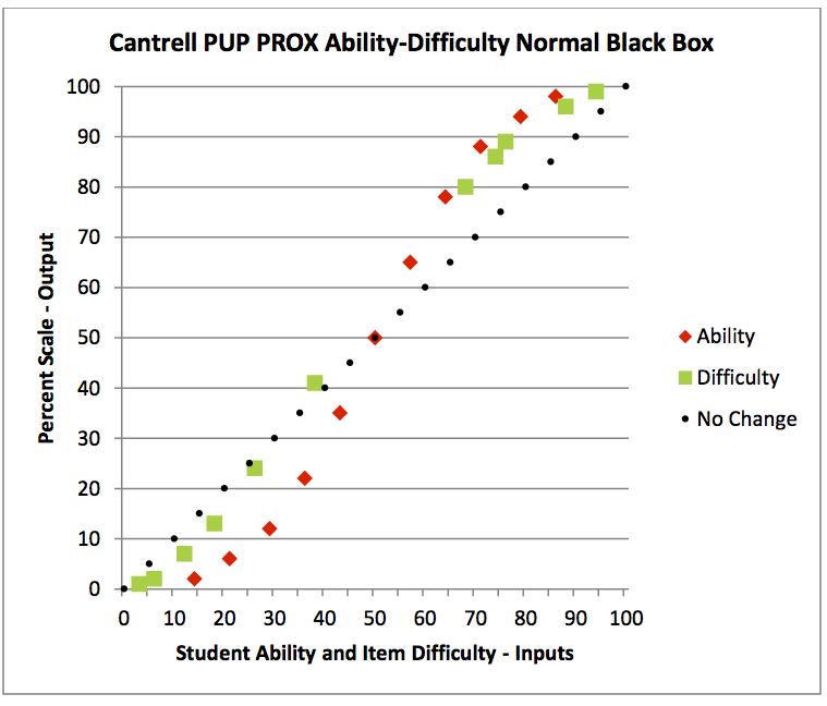
The Cantrell normal PUP PROX conversion from the logit scale throws the student ability distribution into an S-shaped curve. It is still centered at the 50% point.

When the latent student ability locations are being expanded on the logit scale during convergence, they are moving at logit speed (2.718 times faster than normal speed). The farther they are away from zero, the faster they move. The result is a grouping of locations in the outer arms of the normal distribution.

The Cantrell Winsteps data show even greater dispersion after ten JMLE iterations past the PUP PROX data. The zero location is not maintained, and S-shaped curves have now developed in both ability and difficulty distributions. These become even more exaggerated when converted to normal values.

This development of an S-shaped curve results from expanding student ability locations. A chart based on the Rasch model curve shows the effect of expansion from one (no change) to four times. PUP PROX yielded an expansion factor of 2.15 and Winsteps yielded an estimated 3.09. Convergence operations are carried out on a linear logit scale. When converted, the normal student ability results are thrown into an S-shaped curve where the locations clump at the ends of the distribution.

The Nursing1 logit, PUP PROX and Winsteps (PROX & JMLE), results show very different results from Cantrell results. The average test score is 80% rather than 48% (mastery rather than meaningless ranking). Student ability locations are successfully centered on the zero location. Both ability and difficulty distributions are plotted in perfectly straight lines. A difference in average raw score between the two data sets, of 32%, has moved the item difficulty location distribution far away from the zero location. The initial shift of the average input Nursing1 item difficulty logit location was 1.62 logits.

The Nursing1 normal PUP PROX conversion from the logit scale results in a large curve for item difficulty locations and a shallow S-shaped curve for student ability locations. The full nature of the curves was exposed by extending the data.

A linear shift of zero (no change) and 0.5, 1.0, and 1.5 logits of item difficulty locations shows how the curve in the Nursing1 data developed -- the greater the shift, the lower the curve. Item difficulty locations did not migrate toward the ends of their distribution as do student ability locations.

Both PUP non-iterative PROX and Winsteps, iterative PROX and JMLE, produce the desired results when fed good test score data. I can now understand the reason for the many features included in Winsteps to help skilled operators to detect and cull data that does not meet the requirements of the perfect Rasch model.

The Cantrell data do not fit the requirements. This may be part of the reason Cantrell failed to find student ability and item difficulty independence. 

Good data must then have similar distributions (standard deviations). The average test score does not need be near 50% for a good convergence.

I am calling the Nursing1 data a good fit for dichotomous Rasch model analysis based on three observations: 1. Both PUP PROX and Winsteps obtained the same analysis results (non-iterative PROX and iterative PROX:JMLE). 2. The relative location of student ability and item difficulty remained stable from input to output. 3. The logit plot is a perfectly straight line for both student ability and item difficulty locations (considering rounding errors).

Dichotomous Rasch Model Audit

                                                             41

The internal black box audit tool, introduced in the previous post, provides a clear view of what is happening on the logit scale during convergence. Three sets of answer sheets provide the needed data to explore these happenings with average test scores of 80%, 59%, and 48%. These three values as associated with mastery, passing in the classroom, and optimum for psychometric analysis.

Student and Item Data
	Score	Initial Standard Deviation	Number
Nursing1	80:20	0.70:0.95	22:21
EDS - Moulton	59:41	0.97:1.63	9:10
Cantrell	48:52	0.85:2.20	34:14

The Nursing1 chart shows the input values evenly spaced with the exception of a very small ever-expanding distribution. This “error” is an artifact of converting normal values to logit values. The input item difficulty values are shifted to comparable student ability values in an orderly manner, that is, the lines are parallel. The average item difficulty logit value is relocated to zero. This data set represents a good fit to the Rasch model, given my current understanding. The relative positions of student ability and item difficulty remain stable from input to output.

The EDS data shows student ability and item difficulty expanding at two different rates. Here the initial standard deviations differ more than in the Nursing1 data. The result is that the relative positions of student ability and item difficulty changed from input to output.

The Cantrell data are centered near the 50% normal or zero logit location. There was no need to relocate item difficulties, as was done with the Nursing1 data. There was a need to respond to the two very different initial standard deviations. This caused the student abilities to be expanded far faster than the item difficulties.

A second observation on the Cantrell data relates PUP non-iterative PROX and Winsteps results. Winsteps results at four JMLE iterations compared to PUP PROX results. Winsteps then continued ten more JMLE iterations before convergence was called. This both increased the expansion of the distributions but also increased the change in the relative locations of student ability and item difficulty from input to output.

The destabilizing factor seems to be the relative spread of the two distributions for student ability and item difficulty. Statistically the distributions (standard deviations) are being matched, when converging, for the Cantrell and EDS data, but the process changes the relative individual locations.

Good data must then have similar distributions (standard deviations). Also the values need to fall within about -2 to +2 logits (12% to 88% normal).

I am calling the Nursing1 data a good fit for dichotomous Rasch model analysis based on two observations: 1. Both PUP PROX and Winsteps obtained the same results (non-iterative PROX and iterative PROX:JMLE). 2. The relative location of student ability and item difficulty remained stable from input to output.

Rasch Model Convergence Black Box

                                                             40

When this audit started over two years ago, I never planned to travel inside the Rasch model algorithms. Surely by taking a close look from outside (the black box audit tool) one could satisfy that no pixy dust was needed to accomplish the proclaimed feats. The fact that several claims have been discounted in the past ten years, after being applied to NCLB standardized paper tests, makes me question the basic process of estimating item difficulty and student ability measures. (This doubting has nothing to do with the successful application of the Rasch model in many other areas.)

A number of things have raised my doubts. Normal test results cannot be given special value by converting from normal to logit values. The perfect Rasch model is a curve, not a straight line. Laddering across several grades is now in question (in part IMHO because the tests are still scored at the lowest levels of thinking – a guessing exercise -- rather than giving students the option to report what they actually trust – Knowledge and Judgment Scoring). Even some psychometricians still doubt the claims made for the Rasch model.

The black box audit tool that I have been using relates what goes on inside the full Rasch model to the normal world. Conversions of normal to logit and logit to normal add nothing to the audit tool. And nothing has been found amiss. A better audit tool is needed now that we are inside the full Rasch model.

The various ways of estimating student ability and item difficulty measures make use of the original student marks on the test, the student score, the item difficulty, and their distributions (mean and standard deviation). One end result from the transposed Rasch partial credit model is that the estimated individual latent student ability expresses, in one term, what is presented by Knowledge and Judgment Scoring in two terms: quantity and quality. Quantity and quality are directly related to student marks. Estimated latent student ability is dependent upon an estimate of how student marks are related to item difficulty: convergence.

This new black box audit tool relates just these internal values. The two EDS distributions, from the previous post, for student ability and item difficulty, radiate from different starting points and expand at different rates. The span from -2 to +2 logits covers the expected score range from 12% to 88%.

The relative locations for student abilities and item difficulties increasingly change from the positive to the negative regions of the logit scale. This maybe intended or is just an acceptable artifact to psychometricians. It presents a problem for state departments of education that claim their tests are so difficult that passing can be set around 40% on NCLB standardized tests. (I would think this region would be of very little interest in the classroom where the customary passing point is 60% and the average test score is 75%. It is of no interest when hidden by state departments of education by only reporting passing rates without reporting test scores.)

I read the individual student abilities and item difficulties plots, from the internal audit black box tool, to mean that item difficulty is being reported increasingly higher than the comparable student ability, the lower the item difficulty. This would make a test using these items easier than expected in this region, the region of super low cut scores.

Distribution statistics do not reveal individual student and item performances.  Instead they show that, as the item difficulty mean of -0.44 was relocated very near to zero, the student ability mean drifted from 0.39 to 0.71 log its.

The rate of expansion for student ability was larger than for item difficulty. This did little to match the two distributions. The expansion of the two logit distributions was very linear. Yet the end result of the analysis, in normal values, was S-shaped curves.

If the distribution statistics are acceptable, does it matter what happens to individual students? I think so. This is an example of why research techniques do not always work in the application environment.

The best defense students have is to actually know their subject or master the skill to the point that passing is assured. Trying to pass with one point over the line is as flawed a student method as is the state department of education method of setting the cut score before the test is scored to see what actually happened. Application has more serious individual requirements than research.

One auditing method that I have yet to see used is for teachers to include a ranking of their students with the answer sheets. An even better method IMHO is for students to rank themselves by electing Knowledge and Judgment Scoring and reporting what they trust (using all levels of thinking) rather than taking the traditional forced-choice test based on the lowest levels of thinking (meaningless guessing in the cut score region). [Meaningless to everyone except psychometricians only interested in ranking performance.]

Moulton JMLE Example

                                                              39

The EDS Excel example by Dr. Mark H. Moulton is a complete functional solution for latent student ability and item difficulty calibration. However, plugging numbers into algorithms is not the same as understanding what is happening. This JMLE discussion makes use of four of the EDS charts with no missing marks.

The observed raw values chart (Chart 1) is identical to iterative PROX: raw scores are converted into student ability logits [logit = ln(right/wrong)] and items are converted into difficulty logits [logit = ln(wrong/right). Again the item difficulty mean is subtracted from each item to shift the item difficulty distribution to center it on the zero logit location; the first step in converging student ability and item difficulty estimates.

The Rasch model [expected probability = exp(person logit – Item logit)/(1 + exp(person logit – item logit)] is then applied to the raw value chart (Chart 1) marginal logit cells to generate an expected probability value for each internal expected value chart cell (Chart 2). The 0 and 1 for wrong and right in the raw values chart (Chart 1) are replaced with the probability of a student with a given ability being able to mark correctly 50% of the time an item with a given difficulty in the expected value chart (Chart 2).

The marginal logit raw values (Chart 1) control the pattern of the probability values within the expected value chart cells (Chart 2). The variance [variance = probability * (1 – probability)] of expected values chart (Chart 3) has the same cell pattern. Therefore all students with the same score, or items with the same difficulty, receive the same expected probability value and the same variance value.

Subtracting the expected probability values (Chart 2) from the observed raw values (Chart 1)  [0 and 1] fills the internal residuals chart cells (Chart 4) [residuals (Chart 4) = observed (Chart 1) – expected (Chart 2)]. Filling in Chart 4 marginal cells will complete the first JMLE iteration.

The logit distributions expand as the process of convergence progresses. Student ability expands faster than item difficulty. Convergence must not use too large or too small of steps. A scheme is needed that senses the approach of convergence and that makes an expansion step that does not overshoot the point of convergence; where student ability matches item difficulty resulting in a right mark 50% of the time.

The approach of convergence is monitored by first summing the residuals for each person and each item in Chart 4. Some are positive and some are negative. Squaring turns all of them positive. The sum of positive squared person residuals is then used to monitor the approach of convergence; the point when the sum of squared residuals has a value of or near zero.

The last thing we need is to control the size of change made with each iteration. In general the change is something less than the current residual value. The sum of residuals for each person and each item is standardized by dividing by the respective sum of variances for each person and item; this is in contrast to PROX where item variance is applied to person logits and person variance is applied to item logits. The standardized value is then combined with logit measures that are also standardized values. The ninth iteration expansion values (left) are less than one percent of those in the first iteration (right), in this example.

The final step in each iteration is to fill the marginal cells with expanded person and item logit values. The standardized residuals are subtracted from the current person and item logit values. This expands their locations on the logit scale.

The next iteration again fills an expected value chart (Chart 2) using the Rasch model to create new probability values from the old (Chart 4) logit values. Then a new variance chart (Chart 3) and a new residuals chart (Chart 4) complete each iteration.

Again, there is no need for pixy dust but there are still lingering questions. The perfect Rasch model requires near perfect item calibration and latent student ability estimates on a nearly perfect linear scale. The unsettling alternative is a skilled operator who can deliver desired results.

Partial Credit Rasch Model

                                                            38

This post builds on the previous post on the Rasch rating scale model. Three relationships were established:

1.     Students with the same scores and items with the same difficulties were grouped together.

2.     Transposed results for student scores and item difficulties were equivalent to normal results (this is easily seen in the dichotomous Nursing1 data) with identical normal student ability and transposed item difficulty measure means (1.78).

3.     Restoring transposed to normal values and locations required multiplying by -1 and then adding the measures mean (flipping the logit scale end for end and then moving the transposed distribution to the correct location).

The partial credit Rasch model adds to this, the ability to set rating scale thresholds for each item or each student. Now students with the same score can receive different estimated abilities; items with the same difficulty can receive different estimated difficulty calibration values using Fall8850a.data:

1.     A normal partial credit analysis groups student raw scores and treats item difficulties individually (student ability measure mean: 1.24).

2.     A transposed partial credit analysis groups item difficulties and treats student raw scores individually (item difficulty measure means: 1.37).

3.     Restoring transposed partial credit individual student ability measures only imperfectly aligns them with normal individual item difficulty measures (the means are not identical as with the rating scale method: 1.32).

 

The last two charts use rating scale results as a fixed reference, as normal and transposed rating scale means (1.32) are identical from Winsteps. The normal partial credit analysis held person measures an average of 0.08 log its less than the rating scale method as it developed individual item difficulty measures. There is a noticeable curve in the relationship between the two methods.

 

 The transposed partial credit analysis held item difficulty measures an average of 0.05 log its more than the rating scale method as it developed individual person ability measures. The plot is a straight line. The partial credit method can not be directly related to the rating scale method using Fall8850a data.

 

The individual student and individual item measures can be imperfectly aligned by plotting restored transposed student ability measures with normal item measures. The relative locations of student ability and item difficulty do not hold constant as the location of a group is only close to the average of the group. Students (within a group receiving the same test score) with higher IRT ability measures also had higher percent right (CTT quality) scores using Knowledge and Judgment Scoring in PUP. This makes sense.

The item with the fewer number of omits received a higher location (more difficult) on the logit scale than another item with the same count or percent right. This makes sense. An item that more students mark right (and wrong) is more difficult than an item that more students omitted and ended up with the same right count. Also items in a group with higher measures were, in general, more discriminating, PUP 7. Test Performance Profile.

Iterative PROX groups items with the same difficulty. It is in the second stage of Winsteps, JMLE, where items are separated individually. (JMLE replaces each mark with a probability, whereas, PROX only uses the marginal cells of student score and item difficulty.)

Separation is higher for grouped values than for individual values. This relates to the wider dispersion of measures for grouped values. Reliability is the same as from Knowledge and Judgment Scoring. At this point it is safe to say that any study must use only one IRT method to estimate measures. Different methods yield measures that are similar but not identical.