CTT and IRT - Precision

                                                               49

Precision is calculated differently for CTT (CSEM) and IRT (SEE). In this post I compare the conditional standard error of measurement (CSEM) based on the amount of right marks and the standard error of estimate (SEE) based on the rate of making right marks (a ratio instead of a count). It then follows that a count of 1 (out of 20) is the same as a ratio of 1:19 or a rate of 1/20.  Precision in Rasch IRT is then the inverse of precision in CTT in order to align precision estimates with their respective distributions (logit and normal).

Table 45

Table 48

Table 45, my audit tool, relates CTT and IRT using real classroom test results. It does not show the values when calculating the probability of a right mark (Table 45b). I dissected that equation into the difference between ability and difficulty (Table 48a) in measures and in normal values (Table 48b).

Table 49

Table 49 shows the highlights. I found the degree of difference between item difficulties (15, 18, and 21) of 3 was maintained across all student scores (from 14 to 20), 0.81 for 3 counts below the average difficulty of 18, and 1.62 for 3 counts above the average item difficulty (upper right). A successful converge then maintains a constant difference across varying student scores. [Is this the basis for item difficulties being independent from student scores?]

On the average student score (17) the difficulty measures value doubled from 0.81, at 3 counts below the mean, to 1.62 at the mean, and doubled again to 3.24 at 3 counts above the mean (center upper left).

The above uniform expansion on the logit scale (Table 49) yields an even larger expansion on the normal scale. As the converging process continues, the top scores are pushed further from the test mean score than lessor scores. The top score (and equivalent logit item difficulty) of 4.95 was pushed out to 141 normal units. That is about 10 times the value for an item with a normal difficulty of 15 that is an equal distance below the test mean (lower left).

Chart 92

Chart 102

Re-plotting Chart 92, normal scale, on measures (Chart 102) shows how markers below the mean are compressed and markers above the mean are expanded. The uniformly spaced normal markers in Chart 92 are now spaced in increasing distance from left to right in measures in Chart 102.

Chart 103

Chart 104

I sequentially summed each item information function and plotted the item characteristic curves (Chart 103, normal scale and Chart 104, measures). High scores (above 17 count/81%/1.73 measures) with low precision drop away from the useful straight line portion of the Rasch model curve for items with low difficulties (high right score counts). This makes sense.

Chart 91

Chart 105

These item information curves fit on the higher end of the Rasch model as shown in Chart 91. I plotted an estimated location in Chart 105 and included the right counts for scores and items after Winsteps, Table 20.1. [Some equations see actual counts, other equations only see smoothed normal curves.]

Chart 90

Chart 106

Chart 82

Chart 91 from classroom data (mean = 80%) is very similar to Chart 90 from Dummy data (mean = 50%) for a right count of 17. I added precision Dummy data from Table 46 to Chart 90 to obtain a general summary of precision based on the rate of making right marks (Chart 106).  Chart 106 relates measures (ratio) to estimated scores (counts) by way of the Rasch model curve where student ability and item difficulty are 50% right and 50% wrong for each measure location. See Chart 82 for a similar display using a normal scale instead of a logit scale. In both cases, IRT precision is much more stable than CTT precision.

Precision (IRT SEE, Table 46) ranges from 0.44 for 21 items. [50 items = 0.28; 100 = 0.20; 200 = 0.14; and 400 = 0.10 measure (0.03 for 3,000 items.] Only a near infinite number of items would bring it to zero. [Error variance on 50 items = 0.08; 100 = 0.04; 200 = 0.02; and 400 items = 0.01. Doubling the number of items on a test cuts the error variance in half. SEE = SQRT(Error Variance).]

The process of converging two normal scales (student scores and item difficulties) involves changing two normal distributions (0 to infinity with 50% being the midpoint) into locations (measures) on a logit scale (- infinity to + infinity with zero (0) being the midpoint. The IRT analysis then inverts the variance (information) to match the combined logit scale distribution (see comments I added to the bottom of Table 46). The apparent paradox appears if you ignore the two different scales for CTT (normal) and Rasch IRT (logit). Information must be inverted to match the logit distribution of measure locations.

Table 46

The Rasch model makes computer adaptive testing (CAT) possible. IMHO it does not justify a strong emphasis on items with a difficulty of 50%. Precision is also limited by the number of items on the test.  Unless the Rasch IRT partial credit model is used, where students report what they actually know, the results are limited to ranking a student by comparing the examinee’s responses to those from a control group that is never truly comparable to the examinee as a consequence of luck on test day (different date, preparation, testing environment and a host of other factors). The results continue to be the “best that psychometricians can do” in making test results “look right” rather than an assessment of what students know and can do (understand and value) as the basis for further learning and instruction.

Chart 101

* Free Source: Knowledge and Judgment and Partial Credit Model    (Knowledge Factor is not free)

Addendum: Billions of dollars and classroom hours have been wasted in a misguided attempt to improve institutionalized education in the United States of America using traditional forced-choice testing. Doing more of what does not work, will not make it work. Doing more at lower levels of thinking will not produce higher levels of thinking results; instead, IMHO, it makes failure more certain (forced-choice at the bottom of Chart 101). Individually assessing and rewarding higher levels of thinking does produce positive results. Easy ways to do this have now existed for over 30 years! Two are now free.

References:

Culligan, Brent. Date & Location Unknown.  Item Response Theory, Reliability and Standard Error. 10 pages.  http://www.wordengine.jp/research/pdf/IRT_reliability_and_standard_error.pdf

What is the reasoning behind the formulae for the different standard errors of measurement? 3 pages. Downloaded 4/27/2015. http://stats.stackexchange.com/questions/60190/what-is-the-reasoning-behind-the-formulae-for-the-different-standard-errors-of-m

Basic Statistics Review. Standard Error of Estimate. 4 pages. Downloaded 4/27/2015. 

https://www.msu/user/sw/statrev/strv209.htm

CTT and IRT - Scores

                                                              48

[Chart and table numbers in this post continue from Multiple-Choice Reborn, May 2015. This summary seemed more appropriate in this post.]

Before digging further into the relationship between CTT and IRT, we need to get an overall perspective of educational assessment. When are test scores telling us something about students and when about test makers. How the test is administered is as important as what is on the test. The Rasch partial credit model can deliver the same knowledge and judgment information needed to guide student develop as provided by Power Up Plus.

A perfect educational system has no need for an elaborate method of test item analysis. All students master assigned tasks. Their record is a check-off form. There is no variation within tasks to analyze.

Educational systems designed for failure (A, B, C, D, and F, rather than mastery) generate variation in response to test items from students with variation in preparation and native ability (nurture and nature). 

Further there is a strongly held belief in institutionalized education that the “normal” distribution of grades must approximate the normal curve [of error]. Tests are then designed to generate the desired distribution (rather than let students report what they actually know and can do). Too many students must not get high or low grades. If so, then adjust the data analysis (two different results from the same set of answer sheets).

The last posts to Multiple-Choice Reborn make it very clear that CTT is a less complete analysis than IRT. Parts (CTT) cannot inform us about what is missing to make an analysis whole (IRT). Only the whole (IRT) can indicate what is missing (CTT). The Rasch IRT model may shed light on the missing parts not in CTT. The Rasch model seems to be very accommodating in making test results “look right” judging from its use in Arkansas and Texas to achieve an almost perfect annual rate of improvement and to “correct” or reset the Texas starting score for the rate of improvement.

Table 45

A mathematical model includes the fixed structure and the variable data set it supports or portrays. The fixed structure sets the limits in which the data may appear. My audit tool (Table 45) contains the data. Now I want to relate it to the fixed structures of CTT and IRT.

The CTT model starts with the observed raw scores (vertical right mark scale, Table 45a). Item difficulty is on the horizontal bottom scale. These values stored in the marginal cells are summed from the central cells containing right and wrong marks (Table 45a). Test reliability, test SEM and student CSEM are calculated from the tabled right mark data. This simple model starts with the right mark facts.

The Rasch model for scores turns right mark facts (scores) into a natural logarithm of the R/W ratio and a W/R ratio from item right marks (Table 45b). [ln(ratio) = logit] Winsteps then places the mean of item wrong marks on the zero point of the score right mark scale. Now student ability = item difficulties at each measure location. [1 measure = 1 standard deviation on the logit scale]

The Rasch model for precision is based on probabilities generated from the two sets of marginal cells (score and difficulty, blue, Table 45b).  Starting with a generalized probability rather than the pattern of right and wrong marks makes IRT precision calculations different (more complete?) from CTT. The peak of the curve for items is arbitrarily set at the zero location by Winsteps (Chart 100). This also forces the variation to zero (perfect precision) at this location. [Precision will be treated in the next blog.]

I created a Rasch model for a test of 30 items to summarize the treatment of student scores (raw, measures and expected).

Chart 93

Chart 94

Chart 95

Chart 93 shows a normal distribution (BIONOM.DIST) of raw scores for a 30 item test with an average score of 50% and of 80%. The companion normal (right count) distribution for item difficulty (Chart 94) from 30 students looks the same. This is the typical classroom display.

The values in Chart 94 were then flipped horizontally. This normal (wrong count) distribution for item difficulty (Chart 95) prepares the item difficulty values to be combined with scores onto a single scale.

Chart 96

Chart 97

I created the perfect Rasch model curve for a 30 item test in two steps. The Rasch model for scores (solid black, Chart 96) equals the natural logarithm of the ratio of right/wrong [ln(R/W)] in Chart 93. Flipping the axes (scatter plot) produced the traditional appearing Rasch model Chart 97. This model is for any test of 30 items and for any number of students.   

Chart98

Chart 98 shows the perfect Rasch model: the curve, and score and difficulty, for a test with an average score of 50%.  The peak values for score and difficulty are at 15 items or 50% at zero measures. This of course never happens. The item difficulties generally have a spread of about twice that of student 

scores. (See Table 46 in Multiple-Choice Reborn, and the related charts for 21 items.)

Chart 99

Throughout this blog and Multiple-Choice Reborn the maximum average test score that seems appropriate for the Rasch model, as well as comments from others, has been near 80%. Chart 99 shows right mark score and wrong mark item values as they are input into the Rasch model. They balance on the zero point.

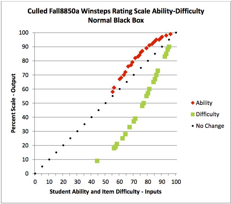
Chart 100

Next, Winsteps, relocates the average test item value (red dashed) to the zero test score location (green dashed, Chart 100). Now item difficulty and student ability are equal at each and every location on the measures scale. I have reviewed several ways to do this for test items scored right or wrong: graphic, non-iterative PROX and iterative PROX.

In a perfect world the transforming line, IMHO, would be a straight line. Instead it is an S-shaped wave (a characteristic curve) that is the best psychometricians can do with the number system used. Both are used in Winsteps Table 20.1. Scores as measures are transformed into expected student scores (Winsteps Table 20.1). In a perfect world expected scores would equal raw scores; there would be no difference between CTT and IRT score results. [For practical purposes, the space between -1 measure and +1 measure can be considered a straight line; another reason for using items with difficulties of 50%.]

Chart 101

* Free Source: Knowledge and Judgment and Partial Credit Model    (Knowledge Factor is not free)

Addendum: Billions of dollars and classroom hours have been wasted in a misguided attempt to improve institutionalized education in the United States of America using traditional forced-choice testing. Doing more of what does not work, will not make it work. Doing more at lower levels of thinking will not produce higher levels of thinking results; instead, IMHO, it makes failure more certain (forced-choice at the bottom of Chart 101). Individually assessing and rewarding higher levels of thinking does produce positive results. Easy ways to do this have now existed for over 30 years! Two are now free.

Rasch Model Student Ability and CTT Quality

                                                              47

How the Rasch model IRT latent student ability value is related to the classical test theory (CTT) PUP quality score (% Right) has not been fully examined. The following discussion reviews the black box results from Fall8850a.txt (50 students and 47 items with no extreme items) and then examines the final audit sheets from normal and transformed analyses. It ends with a comparison of the distributions of latent student ability and CTT quality. The objective is to follow individual students and items through the process of Rasch model IRT analysis. There is no problem with the average values.

We need to know not only what happened but how it happened to fully understand; to obtain one or more meaningful and usefully views. Fifty students were asked to report what they trusted using multiple-choice questions. They were scored zero for wrong (poor judgment), one point for omit (good judgment not to guess and mark a wrong answer), and two points for good judgment (to accurately report what they trusted) and a right answer. Knowledge and Judgment Scoring (KJS) shifts the responsibility for knowing from the teacher to the student. It promotes independent scholarship rather than the traditional dependency promoted by scoring a test only for  right marks and the teacher then telling students which marks were right marks (there is no way to know what students really trust when “DUMB” test scores fall below 90%).

Winsteps displays student and item performance in dramatic bubble charts. The Person & Item chart shows students in blue and items in red. Transposed results (columns and rows become rows and columns) are shown in an Item & Person chart where students are red and items are blue (basically everything has been turned upside down or end over end except the paint job). Blue student 21 with the highest measure (ability) lands as red student 21 with nearly the lowest measure when transposed. That is what is done. Why it is done comes later.

A plot of input/output logit values shows how the process of convergence changes the locations of latent student abilities (log right/wrong ratio of raw student scores) and item difficulties (log wrong/right ratio of raw item difficulties) so they end up as the values plotted on the bubble charts. The ranges of measures on the input/output charts are the same as on the bubble charts. The end over end tipping, from transposing, on the bubble charts also occurs on the input/output charts. Student abilities are grouped as items are treated individually (items with the same test score land at different points on the logit scale). When transposed, items difficulties are grouped as students are treated individually (students with the same test score land at different points on the logit scale). And, in either case, the distribution being examined individually has its mean moved to register at the zero logit location.

The end over end tipping, from transposition, also shows in the normal black box charts. It is easy to see here that the distribution being held as a reference shows little change during the process of convergence. The distribution being examined individually is widely dispersed. Only the highest and lowest individual values for the same grouped value are shown for clarity. Also a contour plot line has been added, for clarity, to show how the individual values would relate to the grouped values if a location correction were made for the fact that all of these individual values have been reduced by the distance their mean was moved to put it on the zero logit location during the process of convergence. In general, the individual values are disbursed about the contour line. This makes sense as they must add up to their original logit mean in the above input/output charts.

The above charts display the values on the final audit sheets for Fall8850a data. Values from Winsteps Table 17.1 Person Statistics were entered in column four Student Logit (+) Output. Values from Table 13.1 Item Statistics were entered in column ten, Item Logit (-) Output. Logit input values were derived from the log right/wrong and log wrong/right ratios for students and items. Normal input values are scores expressed as a percent. Normal output values are from the perfect Rasch model algorithm: exp(logit (+) output)/(1 + exp(logit (+) output)). Normal output (+) item values come from subtracting Normal (-) values from 100% (this inverts the normal scale order in the same way as multiplying values on the logit scale with a -1). One result of this tabling is that comparable output student ability and item difficult values that are clustered together add up to 100% (colored on the chart for clarity). This makes sense. A student ability of 79% should align with an item difficulty with 21% (both with a location of 1.32 logits).

The same thing happens when the data are transposed except, as noted in the above charts, everything is end over end. Column four is now Item Logit (+) Output from Winstep Table 17.1 Item Statistics and column ten, Student (-) Output, is from Table 13.1 Person Statistics. Again an item difficulty of 59% aligns with a student ability of 41% (both with a location of 0.37 logits).

Only normal values can be used to compare IRT results with CTT results. Sorting the above charts by logit input values from individual analyses (right side of each chart) puts the results in order to compare IRT and CTT results. Items 4, 34, and 36 had the same IRT and CTT input difficulties (73%). They had different IRT output values and different CTT quality (% Right) values. The item difficulty quality indicators change in a comparable fashion. (Normally a quality indicator (% Right) is not calculated for CTT item difficulty. It is included here to show how both distributions are treated by CTT and IRT analyses.)

CTT and IRT Quality Indicators
Method	Item (73% Input)
	34	4	36
CTT	83%	85%	93%
IRT	44%	46%	56%

Sorting the transposed analysis by input values groups student abilities. Four students had the same IRT and CTT abilities (70%). They had different IRT output values and CTT quality (% Right) indicators. The point is that these quality indicators behaved the same for student ability and item difficulty and for normal and transposed analyses. 

CTT and IRT Quality Indicators
Method	Student (70% Input)
	26	37	40	44
CTT	81%	88%	88%	95%
IRT	43%	51%	51%	63%
IRT + Mean	68%	76%	76%	88%

These quality indicators cannot be expected to be the same as they include different components. CTT divides the number of right answers by the total number of marks a student makes to measure quality (% Right). The number of right marks is an indicator of quantity. The test score is a combination of quantity and quality (PUP uses a 50:50 ratio). Winsteps combines IRT student ability and item difficulty, with the Rasch model algorithm, during the JMLE analysis into one expected value, at the same time, it is reducing the output value by the distance the mean location must be moved to the zero location point: convergence. CTT only sees mark counts. The perfect Rasch model sees student ability and item difficulty as probabilities ranging from zero to 1. A more able student has a higher probability of marking right than a less able student. A more difficulty item has a lower probability of being marked right than a less difficult item. This makes sense. A question ranks higher if marked right by more able students. A student ranks higher marking difficult items than marking easier items.

The chart of student ability, from normal and transposed analyses, plots the values for the students in the above table scoring 70% on the test. By following up from 70% Input you encounter 43, 51, and 63% transposed individual values below 76% for the grouped non-transposed value. 

The above selection of students and items was made from a PUP Table 3c. Guttman Mark Matrix. The two selections represented uneventful sets of test performances that seemed to offer the best chance for comparing IRT and CTT. PUP imports the unexpected values from Winsteps Tables 6.5 and 6.6 to color the chart. Coloring clearly shows the behavior of three students who never made the transition from guessing at answers to reporting what they trusted: Order 016, Order 031, and Order 035 with poor judgment scores (wrong) of 24, 13, and 26.

In conclusion, Winsteps does exactly what it is advertised to do. It provides the tools needed for experienced operators to calibrate items for standardized tests and to equate tests. No pixy dust is needed. In contrast, PUP with Knowledge and Judgment Scoring produces classroom friendly tables any student or teacher can use directly in counseling and in improving instruction and assessment. Winsteps with the Rasch partial credit model can perform the same scoring as is done with Knowledge and Judgment Scoring. The coloring of PUP tables provided by Winsteps adds more detail and makes them even easier to use.

There is no excuse for standardized tests and classroom tests being scored at the lowest levels of thinking. The crime is if you test at the lowest levels of thinking you promote classroom instruction at the same level (please see post on multiple-choice reborn). This holds for essay, report, and project assessment, as well as, for multiple-choice tests. The Winsteps Rasch partial credit model and PUP Knowledge and Judgment Scoring offer students a way out of the current academic trap: learning meaningless stuff for “the test” rather than making meaningful sense of each assignment that then empowers the self-correcting learner to learn more. The real end goal of education is developing competent self-educating learners. It is not to process meaningless information that is forgotten with each “mind dump” examination.

Personal computers have been readily available now for more than 30 years. Some day we will look back and wonder why it took so long for multiple-choice to be scored, as it originally was before academia adopted it; in such a manner that the examinee was free to accurately report rather than to continue an academic lottery used to make meaningless rankings.

Rasch Model Convergence Normal Black Box

                                                             46

The normal black box displays IRT results on a normal scale that can be compared directly to CTT values. The four charts from Fall8850a.txt, rating scale, culled rating scale, partial credit, and culled partial credit at not too different from the logit black box charts in the prior post. The un-culled data set included 50 students and 47 items. The culled data set included 43 students and 40 items (7 less outlying students and items each).

The first three charts show student abilities passing through the 50%, zero logit, point. Failure for this to be the case with culled partial credit was observed in the prior logit black box post, but is very evident in this normal scale chart. The culled partial credit analysis passed through three iterations of PROX rather than two for the other three analyses.

A curious thing was discovered when developing the extended normal values for student abilities. Up to now all extended student ability estimates only involved multiplying the log ratio value of student raw scores by an expansion factor. For the culled partial credit analysis, a shift value had to be included, as is normally done when estimating item difficulty values. A shift value was not needed when estimating student ability values with the un-culled partial credit data set, or any other data set I have examined. The plot of the extended student abilities would not drift away from the no change line without the additional shift of 0.4 logits.

Student scores are used as a standard in non-transposed analyses. The un-culled data set, using partial credit analysis, will now be used in a transposed analysis where item difficulties become the standard for the analysis. This may clarify the relationship between the quality and quantity scores from Knowledge and Judgment Scoring for each student and the single latent student ability value from Rasch IRT.

Rasch Model Convergence Logit Black Box

                                                             45

This view of Fall8850a.txt Winsteps results has been visited before. The difference is that now I have an idea of what the charts are showing in three ways:

1. The plot of student abilities for the rating scale analysis passes directly through the zero logit location indicating a good convergence. 2. The plots for student abilities and item difficulties are perfectly straight lines (considering my rounding errors), which again shows a good convergence. 3. The two lines are parallel, another indicator of a good convergence.

Culling increased the distribution spread to higher values for both analyses, as shown in the previous post. The plot of student abilities for culled partial credit did not pass through the zero logit location. Removing 7 students and 7 items has resulted in a poor convergence.

The item difficulty plots for the partial credit analysis are very different from those from the rating scale analysis. Here items starting convergence with the same difficulty can end up at various ending locations. The lowest and the highest locations are plotted for each item.

This post must end, as a comparison of Rasch IRT and PUP CTT results cannot be made directly between logit and normal scale values. 

Rasch Model Logit Locations

                                                              44

Student ability and item difficulty logit locations remain relatively stable during convergence when using data that are a good fit to the requirements of the perfect Rasch IRT model. The data in the Fall8850a.txt file requires that the average logit item difficulty value be moved one logit, from -.98 to 0, during convergence. The standard deviations for student ability and item difficulty, 0.51 and 1.0, are also quit different.

The relative location of individual student abilities and Item difficulties vary, from the two factors above and from the culling of data that “do not look right”, during the process of convergence on the logit scale. Individual changes in the relative location of student ability and item difficulty can be viewed by re-plotting the bubble chart data shown in the previous post.

The rating scale analysis groups all students with the same score and all items with the same difficulty. The end result is a set of nearly parallel lines connecting the starting and ending convergence location of a student or an item. (Closely spaced locations have been omitted for clarity.)

Culling outliers resulted in the loss of values among the less able students and the more difficult items.

This increased the student ability mean and decreased the item difficulty mean. Culling increased the spread of both distributions toward higher values.

The partial credit analysis groups all students with the same score but treats item difficulty individually. (More locations have been omitted for clarity.) Four of the plotted starting item difficulty locations land at more than one ending convergence location. Culling partial credit outliers had the same effects as culling rating scale outliers (above) related to where the culling occurred, the migration of means, and the direction of distribution spread. (More item difficulty locations were omitted for clarity.)

The item difficulty mean migrated to the zero logit, 50% normal, location in all four analyses: full rating scale, culled rating scale, full partial credit, and culled partial credit. Winsteps performed as advertised for psychometricians .

The individual relative locations for student ability and item difficulty differ in all four analyses. Two items, that survived my culling and omitting, have the same starting location but very different ending locations: Item 13 and Item 41. Both are well within the -2 to +2 logit location on the Winsteps bubble charts (item response theory – IRT data).

PUP lists them as the two most difficult items on the test (classical test theory – CTT data). PUP lists Item 13 as unfinished, with 15 out of 50 students marking, of whom only 5 marked correctly. There is a serious problem here in instruction, learning, and/or the item itself. Item 41 was ranked as negatively discriminating (four of the more able students in the class marked incorrectly). Only 5 students marked item 41 and none were correct. The class was well aware that it did not know how to deal with this item. Both items were labeled as guessing.

IRT and CTT present two different views of student and item performance. The classroom friendly CTT charts produced by PUP require no interpretation for students and teachers to use directly in class and when advising.