Benchmark Test

Next      Back     Start              Chapter 17

The benchmark test is the standard for all future tests. It is constructed from calibrated questions and, generally, includes a set of common items. It has been administered at least once to verify that it satisfies statistical expectations. When scored by only counting right marks, the expectations only include the ranking of each item and each student.  The analysis says little about the validity of the test to assess what students trust they know, as the basis for future instruction and learning, or for future job performance.

Calibrated questions are obtained by administering new questions to comparable groups of students.  Field-testing presents a new set of questions to students without consequences. This is a common way to start the process of standardization. Operational testing presents new questions embedded in a test that has consequences, for more valid results. Winsteps estimates individual student ability and item difficulty measures. The measures are reported to provide sample-free item calibrations.

Bookmarking is the practice of placing calibrated questions in a book in an order of increasing difficulty. Experts and judges examine each question to find the one a student must answer to pass the test, a very political process. The outcome has been highly variable (as it is impossible for those with full knowledge to guess what answers students with incomplete knowledge will mark). The average judged item difficulty of the selected questions sets the raw cut score for the test.

Classroom tests, unlike standardized tests, include everyone and everything. PUP Table 7 lists Mastery, Unfinished, and Discriminating (the questions normally used in standardized tests). Even a classroom test can yield high test reliability (>0.90 KR20) if enough discriminating questions are included.

Reporters were concerned last year by the proximity of the random guessing score and the cut score.  Ministep, implementing the Rasch model, does not recognize guessing. This gives students a handicap of 25% on 4-option questions. (I customized PUP, PUP7, to handle 7-option questions, a 14% handicap, last year for a faculty member with a cheating problem from answer copying.)

Winsteps performs as advertised estimating student and item measures, but it has no magic to correct errors in judgment in creating the standardized test, managing drift, and in setting cut scores. Time for testing places a limit on the number of questions on the benchmark test. The main goal of Winsteps is to help select the minimum number of questions that will yield acceptable test reliability.

Next    Back    Start

Common Item Equating

Next    Back    Start                  Chapter 16

Most standardized tests include a small identical set of questions called common items. The idea is that the common items set a standard of performance. If the average performance of the common (C) items is the same when attached to Test A and to Test B, then Test A and Test B are equivalent tests. If the common items differ, then one test can be adjusted, equated, to fit the other test’s frame of reference.

The 24 by 24 question-student test was divided into two sets of nine questions (Test A and Test B) and one common set of six items that covered the range of difficulties. The estimated difficulty measure for each common item varied from test to test:  A, B, C, and AB. The average measures of the six common items also varied from test to test. This variation may not occur with Winsteps when using hundreds of answer sheets. 

A ratio near 1.0 of the common item average measure standard deviations from Test B/Test A indicates the two tests performed in a similar fashion and can be equated. Excel returned a standard deviation Test B/Test A slope of 1.26/1.30 or 0.97 for the common items included in Test A and Test B. A perfect match would require not only a close match of standard deviations, but also of the other distribution characteristics: mean, mode, median, skew and kurtosis.

The difference in the location of the common items for Test A and Test B, each with 15 items, is related to Test A average measures (0.20) being estimated less difficult then Test B average measures (0.56). The related test scores were 80% for Test A and 84% for Test B. The easier the test the higher the estimated matching item difficulty and student ability measures

Test B measures are put into the frame of reference of Test A by reducing Test B measures by the average of Test B common measures and then adding the average of Test A common measures. The correction factor (- Test B average + Test A average) is -0.56 + 0.20 or -0.36.  Adding -0.36 to each Test B measure puts it into the frame of reference of Test A. This is the same as sliding one Table 1.0 person-item map past the other in the [previous] blog, which produced a confirming value of -0.33.

In either case, graphed or calculated, one collective group correction factor (that is most reliable near the mid-range on the scale) is applied to each individual item difficulty measure. This same practice of applying a group correction factor to individual statistics occurs in traditional item analysis, classical test theory (CTT), as on PUP Table 7 Test Performance Profile.

Next     Back     Start     

Simple Virtual Equating

Next    Back     Start               Chapter 15

Another simple method of equating involves printing out Ministep Table 1.0 for each test and then sliding one along side the other until they are in reasonable agreement. This post also introduces six equally spaced common items in preparation for common item equating. The 24 by 24 student/item nursing school test was divided into two sets of nine items and one set of six common items. This produced two 15-student by 24 item tests (A9C6 and B9C6).

The average measure for the six items selected as common items was zero, that is, they were indeed uniformly distributed on the linear logit scale.

Winsteps Table 1.0 printed out with 12 divisions between each measure for both Test A and Test B. The spacing was identical for the two tests between -2 and +3 logits. The six common items can be identified by their answer sheet code, x2x, plus the item number: x2x 4. Winsteps Table 1.0 is a uniform linear playing field.

Without using the six common items, you must slide Test B vertically past Test A until “the overall hierarchy makes the most sense”. With the common items, you slide until the common items are in a best registration location. “The relative placement of the local origins (zero points) of the two maps is the equating constant.”  (The student ability zero points on the two tests also come together. This makes sense as equivalent student ability and item difficulty have been plotted at the same points on this linear logit scale.) 

In my judgment, the distance between the Test A and Test B item zero points is about 4 divisions x 1/12 logits or -0.33 logits.    

Test A was more difficult than Test B. The constant -0.33 can now be added to Table 13.1 measures in Test B. Test B 2.10 + (-0.33) = Test A 1.77. Equating reduces Test B student ability and item difficulty measures when placed within the Test A frame of reference.

This post presents a visual view of what equating involves. A single constant can be added to all measures, to equate two tests, as the measures are now on a linear logit scale. This constant is calculated when using [common item equating] rather than judging the value as above.[link next]

Next      Back    Start           Download  PUP Answer Data for Ministep

One-Step Equating

Concurrent or One-Step Equating

Next      Back     Start            Chapter 14

This is the simplest method of equating two tests. It puts all the data into one file. The Rasch model requires that the two sets have matching characteristics.

Two sets came from splitting the 24 by 24 student/item nursing school test into two 12-student by 24-item tests (A and B). Each was analyzed by Ministep.

Crossplotting values, from Winsteps Table 13.1 Items, verified that the two sets performed similarly, with Item difficulties from Test B on the vertical axis and from Test A on the horizontal (y = 09861x + 0.0484 = 1.03). Also the ratio of standard deviations (S.D.) or slope was B (1.34)/ A (1.28) = 1.05. Any value near one is acceptable.

Excel and Winsteps produced the same slope value. Excel produced a higher S.D. (1.37 instead of 1.34 on Group B) as Excel makes a correction for the small number of items.

The S.D. ratio near one is an indicator that the two tests are performing in a similar manner, not a determination that they are exactly alike. There are other statistics that complete a fuller view than just using S.D.

The values for median (half way between extremes) and mode (most frequent tally) are of little use with samples of only 12 students and 24 questions, illustrated on the Estimated Item Difficulty chart above, except to indicate that the data are skewed (mean, median and mode are not the same). Group B has almost no skew (0.05).

A value of one for kurtosis indicates the sample fits the relative height of the normal curve. Group B is very flat (-1.31). Four of the five Group B plot points are about the same height on the Item Difficulty Distribution chart. Most striking on this chart is that when two small sets of very similar data (A and B) are combined, the result (C) takes on a much different appearance. A 24 by 24 student/item matrix (about 500 data points) is near the minimum requirement for both Winsteps and PUP. Part of the change in appearance is captured in maximum, minimum and range (see top chart). All of these statistics deal with the characteristics of group performance rather than individual student or item performance.

There is a need to keep in mind, what these basic statistics capture in numbers, as an overall perspective to specific analyses. Winsteps captures individual estimated student ability and item difficulty measures. PUP captures what individual students trust they know and their ability to use what they know: quantity and quality (with Knowledge and Judgment Scoring). Once these numbers have been obtained they are easily manipulated. Many different stories can be told from the same data, especially when students are not permitted to exercise their own judgment in reporting what they trust, on paper tests and with computer adaptive testing (CAT).

Next    Back     Start

Test Characteristic Curve

Next     Back    Start                        Chapter 13

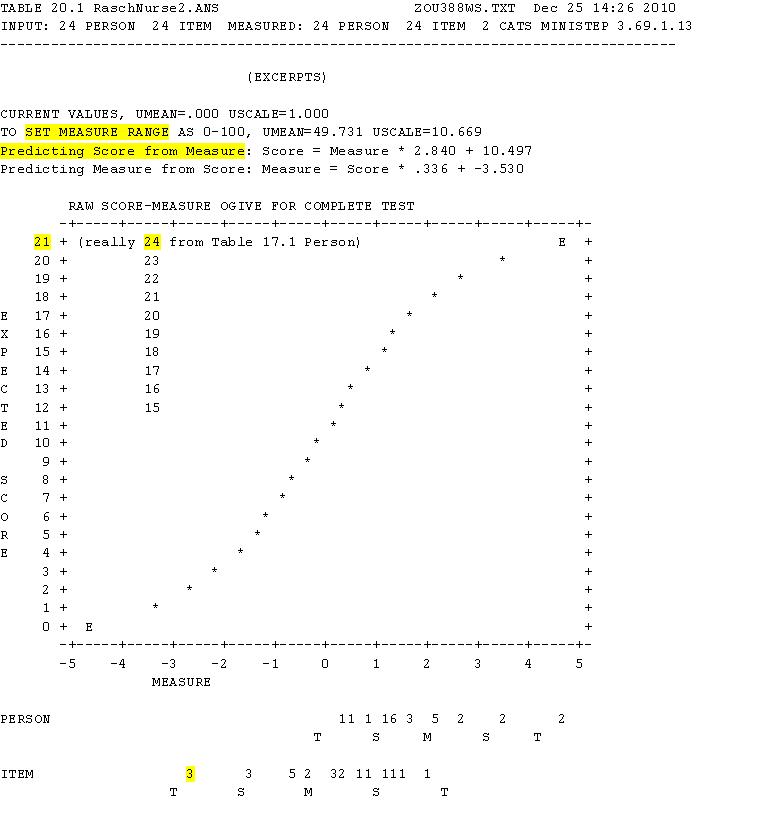
The test characteristic curve (TCC) is used to relate one test with another. Ministep Table 20.1, Raw Score-Measure Ogive for Complete Test, displays the TCC and the expected raw scores when student ability measures equal item difficulty measures.

The TCC results from Winsteps processing observed student test scores into estimated measures and then predicting expected student raw scores. 

Table 20.1 assists in predicting raw scores from estimated measures and the reverse (mapping). This relationship is fully linear rather than an ogive. Values are also presented to assist in setting the range of scaled scores, of replacing the unit for measures (the logit) with arbitrary values.

Winsteps has a problem with questions and students who generate perfect scores. The TCC in Table 20.1 terminates with 21 rather than 24 as all students marked three items correctly. Perfect scores are rare when using several hundred answer sheets. Other factors influence the TCC and it use.

Winsteps uses “fit” to describe how well persons and items match the Rasch model requirements. PUP uses “fitness” to describe how well the test matches student preparation. The fitness value is also called the average student educated guessing score. It has a value of 100% on a perfect test (a check list of what students have mastered). Fitness has a value of 25% on a 4-option multiple-choice test where all options are about equally marked. This would be a very difficult test, requiring considerable guessing when forced-choice scoring.

The average student educated guessing score ranged between 38.7% and 55.8%, on PUP Table 5, with an average of 47.8%. About half of the answer options on the test could be discarded by students functioning at higher levels of thinking before selecting their “best” right answers.

Guessing is not a part of the Rasch model. With test fitness near 50%, and an average test score of 84%, guessing had little effect on the scores of this test. Guessing can have a marked effect on test scores when test fitness drops to the design level of 25% for 4-option questions. At this point the Rasch model and the three-parameter (3-P) IRT model, that includes guessing, diverge widely.

Forced-choice or guess testing requires a mark on each question. Knowledge and Judgment Scoring (KJS) only requires a mark to use a question as a means of reporting what a student actually knows or can do (what is known and the judgment to correctly use what is known). The Rasch model labors under the requirement for students to guess just as with traditional, right mark, scoring. The partial credit Rasch model may serve KJS better.

Next    Back    Start

Person Item Map

Next   Back   Start                        Chapter 12

 

Ministep Table 1.0 combines the data in Table 13.1 Person, and Table 17.1, Item, into a second visual display of test results (also see bubble graphic). Estimated student ability and item difficulty measures are placed side by side, in one vertical dimension, and in the same sequence as the normal distributions are on PUP Table 3 in two dimensions.

The normally distributed test scores (right marks) and difficulties (wrong marks) have been edited into Table 1.0 to again show the difference between the two distributions (normal and logit). The logit scale suggests that it takes more effort to move from a score of 22 to 23 than from 15 to 16.

Winsteps Table 1.0 shows which students and questions match on an estimated student-ability:question-difficulty measure scale. The most efficient testing is done with items and students that have similar estimated measures.

The Rasch Model is therefore a common method for calibrating test items for use in computerized adaptive testing (CAT). After each examinee’s forced response to a question, the computer quickly calculates the expected range of success for this student and delivers a more difficult one if the response was right and an easier one if the response was wrong. The test ends when the score falls within, or without, preset confidence limits or the maximum number of questions or time is reached.

Healy, Nicho, and Summi, estimated person measure of 1.73, can be expected to earn a score of 85% on items with an estimated difficulty measure of zero (=exp(Ability-Difficulty)/(1+(exp(Ability-Difficulty)) or exp(1.73 - 0)/(1+exp(1.73 - 0)) or exp(1.73)/(1+exp1.73) or 5.65/(1+5.64) or 5.64/6.64 or 0.85 or 85%). This makes sense, as the average test score and item difficulty were 84%.

Insert your choice of ability and difficulty into the Rasch model to predict expected raw scores on future tests. Salto (or a group of students with Salto’s ability), estimated person measure of 0.34, can expect to answer 20% of items correctly that have an estimated difficulty measure of 1.73 (=exp(0.34 – 1.73)/(1+(exp(0.34 – 1.73)). Salto also has a 20% or 0.2 chance of answering correctly any one question with a difficulty measure of 1.73. CAT would use some easy questions to assess Salto. They could be like the questions on this test.

Next     Back      Start

Rasch Estimated Measures

Next    Back    Start                        Chapter 11

Deep within the Rasch model is the mystery of how person and item normal scales are combined into one logit scale. Ministep starts with a typical data matrix, such as PUP Table 3.

Question difficulty is converted from the number of right marks to the number of wrong marks in Step 1.  The average difficulty of 84% right is now expressed as 16% wrong.

The cells recording right and wrong marks in PUP Table 3 are converted to probabilities. The marginal cells, in Table 3, for student score and question difficulty are converted from normal to logit values in Step 2.

The initial location of student scores and question difficulty ranges from  nearly -5 logits to nearly +5 logits for the student nurse test results on PUP Table 3. 

In Step 3, the final location for estimated student ability and item difficulty measures results when the item difficulty measure of zero (0) logits rests below the normal average student score (84% right). The normal average test item difficulty (16% wrong) rests below the student ability measure of zero (0) logits.

     --------0--------------84%------- person ability 

----------16%-------------0-----       item difficulty 

Equivalent means are in registration. They mark off equivalent lengths (1.66 measures) of the logit scale on this test.

This is not just a case of shifting the item tally past the ability tally, but a re-plotting of the item values onto a single logit scale. Re-plotting compressed the negative item measure locations by 0.84 and expanded the positive item measure locations by 1.16 to create a close fit to the Winsteps Person-Item Bar Chart.

There are many ways to set person and item final locations, the basis for the test characteristic curve (TCC). Winsteps uses two methods in series, normal approximation algorithm (PROX) and joint maximum likelihood estimation (JMLE). For this test it cycled through PROX twice and then through JMLE twice.

Next    Back    Start