Non-Iterative PROX and Winsteps

                                                            33

Winsteps ignores extreme values (when all students mark the right or wrong answer on an item or a student marks all right or wrong answers on all items on the test) when estimating measures. Winsteps prints extreme values in the student and item reports and on the person-item bar chart (100% is replaced with a bit smaller number). This makes the reports convenient for classroom use, but prohibits comparison of black box input-outputs from different methods of estimating measures, unless extreme values are deleted prior to running Winsteps.

[UEXTREME=Yes has just been added to Winsteps 3.74.0 to include extreme values, 15 April 2012, as I am writing this.] The PROX routine in Power Up Plus 5.10 (PUP) deletes extreme values so no manual cleanup is needed.

Data from the 24-student by 24-item Nursing1 test was selected to compare non-iterative PROX and Winsteps. PUP Table 10 shows 22 students and 21 items remaining after excluding extreme values. The average test score for these students, preparing for a standardized test, was 80%.

The sequence of student ability and item difficulty plots, for PROX and Winsteps, in every case, appear in order at a resolution of 1/10 measure. Sixteen of the twenty points are identical for the two methods of estimation. There is little question that corresponding student ability and item difficulty values are being accurately plotted.

The black box charts show that the mean for item difficulty was successfully moved to the 50% (zero logit) position by both methods for estimating measures. This required a shift (-1.62 logit) and an expansion factor (1.11 logit) for PROX. The average input value (20%) was changed to an average output value of 50%, a change of 30% when converting the negative item count to a positive student expected score.

Student ability changed very little as only the expansion factor (1.18 logit) was applied by PROX. Winsteps had to make similar changes in its two-stage estimation.

Non-Iterative PROX Algorithm

                                                              32

(Single-cycle Rasch model measures estimation)

How student scores and item difficulty can be re-plotted onto one scale was considered graphically in Rasch estimated measures. The item difficulty mean was placed in register with the student ability zero location on the logit scale. The item difficulty zero location was then in register with the student ability mean location. Equivalent portions of the scale for the two distributions (item to student: mean to zero and zero to mean) were in register with one another.

This same thing can be done by capturing the required properties in numbers. These estimates can be made with PROX for a data set with no missing marks. (This is no problem using traditional right count scoring when omits are scored as wrong.) Catherine E. Cantrell published in 1997 the step-by-step calculations for PROX.

These estimates are summarized in PUP Table 10. The table lists values for right and wrong counts, and ability and difficulty measures. The table provides an insight into how PROX performs. It is the source for several charts.

[Plotting the tally column by the expanded measures columns yields the student ability–item difficulty (Winsteps bar) tally. Plotting the black box output column (Winsteps expected student scores) by the expanded measures columns yields the test characteristic curve (TCC). And plotting the output columns by the input columns yields the black box audit tool that is responsive to all changes made.]

PROX makes a tally of the student right mark counts and the item wrong mark counts (columns one and seven). The observed scores are converted into natural log ratios (right/wrong for score ratios and wrong/right for item ratios) to obtain a nearly linear logit scale.

Now to shift the item difficulty mean to the student ability zero location on the logit scale. The logit scale starts at zero and radiates in either direction (-5 to +5 in this example). The initial item measure mean was 0.22 logits. This is subtracted from each item difficulty measure (column 9) to shift the item difficulty measure distribution into register with the student ability measure distribution (as was done graphically in Rasch estimated measures).

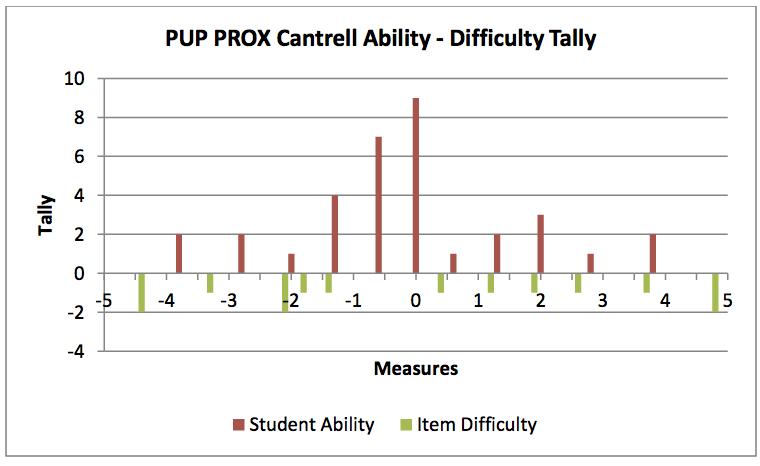
The final step is to apply an expansion factor. It is based on the variance within student score and item difficulty measures. The expansion factor chart shows that as the standard deviation for item difficulty grows, the greater is the resulting expansion factor. In general, the expansion factor for ability is about twice that for difficulty. It is normal for item difficulty to spread out in a wider distribution than student ability scores.

The expansion factor for student ability is obtained for PROX by taking the square root of the ratio of the variance within item difficulty measures (U) to the product of the variances for student ability and item difficulty measures. The expansion factor for item difficulty is based on the ratio of the variance within student ability measures (V) to the product of the same two variances.

After adding in constants to match the logistic and normal distributions (1.7, 2.89 = 1.7 squared, and 8.35 = 2.89 squared) the expansion factors become SQRT((1+(U/2.89))/(1-((U*V)/8.35))) for student ability and SQRT((1+(V/2.89))/1-((U*V)/8.35))) for item difficulty measures. The expand (expanded) table columns are the products of the student ability logit values or item difficulty shift values and their respective expansion factors.

[Multiplying pools the source variances U and V. Dividing their variances by the pool assigns a portion to each source. The larger portion is applied to the smaller source (which is normally the student score distribution). The expansion factors increase the spread of the ability and difficulty measure distributions each way (+ & -) from the zero measure location. The entire PROX process for estimating measures includes simple math and no pixy dust.]

The student ability and item difficulty expanded values are plotted on the ability-difficulty tally chart. The goal is, to have a student ability to mark a correct answer 50% of the time, match an item with a difficulty of equal magnitude. By definition this happens at the zero logit (measure) location. Does this continue to occur as one moves further away from the zero logit location?

Cantrell, Catherine E. (1997). Item Response Theory: Understanding the One-Parameter Rasch Model. 42 p. Paper presented at the Annual Meeting of the Southwest Educational Research Association (Austin, TX, January 23, 1997). EDRS: ED 415 281. 

PUP Quality and Winsteps Measures

                                                             31

The clicker data reviewed in Scoring Clicker Data and Grading Clicker Data provide further insight into Winsteps. The chart in Grading Clicker Data shows how each individual student fairs when electing either right mark scoring (RMS) or Knowledge and Judgment Scoring (KJS). That is an applied student view, a rather busy messy one. The grade chart can be simplified by returning to related scores from RMS and KJS.

The above presentation can be further simplified  by removing duplications. It now only relates the scores obtained from the two methods of scoring, RMS and KJS.  

KJS scores are composed of a quantity score and a quality score; percent of right marks on the test and percent right of marked items; knowledge and judgment. The exact same values are available from Power Up Plus (PUP) and from Winsteps Table 17.1. [RMS = RT/N; Quality Score = RT/(RT + WG); and KJS = (N + RT - WG)/2N] But how are these scores related to measures?  

This chart shows total RMS scores related to measures. This chart prints directly from Winsteps (Plots/Compare Statistics: Scatterplot). This presentation is very similar to the above chart that relates RMS scores to KJS quality scores. Measures are calculated on the number right out of the number marked as are quality scores. Are PUP quality scores and Winsteps measures reporting the same thing?  

This scatterplot shows they are the same but not in the same units. Again we have the situation of buying melons by count at $2 each or by measure at 10 cents a pound. High quality students, who can trust what they know, also exhibit high ability in measures.  

The student showing a KJS quality score of 100% (two right out of two marked) is also the student showing the highest full credit ability measure.  The student with the lowest quality score, one right out of 17 marks, also has the lowest full credit ability measure.

Given the above discussion, it then follows that estimated student ability measures from full credit and partial credit scoring show the same relationship as the KJS quality scores do to KJS student test scores in Scoring Clicker Data. The four students with zero test scores are not included in the Winsteps chart as zeros have no usable predictive value. So, the full credit student ability measure is comparable to the KJS quality score. The partial credit student ability measure is comparable to the KJS student test score.  

The final chart, in this second end of audit posts, relates the estimated item difficulty measures from full credit and partial credit scoring. They are in very close alignment. Even though students receive very different scores and grades from the two methods, the item difficulty remains the same with the exception of the effect of scale on the results. The full credit estimates are based on total counts of 23. The partial credit estimates are based on total counts of 46. A bit of shift and stretch (mean – mean and SD/SD) can bring these two distributions into agreement.  

In conclusion, Winsteps is optimized to calibrate item difficulty for test makers. PUP is optimized to direct student development from passive pupil to self-correcting scholar. Winsteps estimates student ability (measures) to perform on the test (when students are forced to mark every question as is generally done). It estimates student ability (measures) to report what can be trusted as the basis for further learning and instruction when using the partial credit Rasch model (scores identical to KJS).

Both RMS and the full credit Rasch model, that Winsteps is normally used in, suffer from the sampling error created at the lower range of scores where pass/fail cut points are usually set: Even an average “C” student can obtain a “B” one day and a “D” on  another day. Half of the students near the pass/fail line will fall on the other side on the next test with no indication of quality. KJS is a simple solution to this problem as well as a means of directing student development rather than working with questionable student rankings.

The power of self-assessment is lost when students are treated as a commodity rather than as living, learning, self-actualizing beings. A right answer from a person, who has no interest in, places no value on, or sees no connection between facts and observations on the topic has an entirely different meaning than a right answer from a person who is interested in, places a high value on, or sees a web of meaningful relationships between facts and observations. One shows awareness, the other can do and apply. KJS and the partial credit Rasch model can sense this difference in quality. Both incorporate it into the test score. PUP prints it out as a quality score for student counseling and instructional management.

Winsteps - Score Distributions

                                                             30

Winsteps requires score distributions to be very similar to fit the Rasch model when equating. You can do two things to a distribution of scores. You can shift the location of the distribution by subtracting from or adding a constant to each measure, or you can stretch or shrink the distribution by multiplying or dividing with a constant. Winsteps uses one or both of these adjustments when equating.

It is impractical, impossible, to have one set of students mark answers to all of the questions needed for a test bank on one test. This problem is solved, in theory, by administering several tests. Each test contains a set of common items. In theory, these common items will be equally difficult on every test.

Score distributions have many statistics: mean, median, mode, skew, kurtosis and standard deviation (SD). Winsteps uses the SD as the most meaningful way to compare distributions. Combine two very similar distributions (the common items SD of test A/SD of test B is near 1) by shifting the mean of one distribution to match the other distribution. A constant is added to or subtracted from each measure to put test B into the frame of reference of test A.

If the two distributions are not very similar, extreme items can be liberally discarded to obtain a better match for Winsteps in estimating Rasch model measures. This is not directly comparable to discarding values based on right mark counts using CTT. Counts and measures are not the same thing (see previous post).

Winsteps reports student raw scores in perfect alignment with student abilities, Table 17.1. But it reports item difficulties in a fuzzy array, Table 13.1. A range of item difficulty raw score counts can yield the same measure. Two difficult items can be worth the same as three easy items in measures.  

If the two distributions are still not very similar, they can be combined by both shifting the mean, as above, and by stretching or shrinking. The ratio obtained by dividing the common item SD for one test by the other is the required constant. Measures in one of the distributions are multiplied or divided by this constant to put them into the frame of reference of the other distribution.

When to add or subtract, or to multiply or divide, is determined by what activity you are engaged in (item calibration, test banking, cut score, or application) as well as how the two test score distributions match. Psychometricians tend to think along the line that they are sampling from one big population when calibrating items and when applying the standardized test. Many statistics are set up with the normal curve, the know-nothing curve (the curve obtained by marking the answer sheet without looking at the test), as the background reference. (This idea is mostly false in NCLB standardized testing where there is a strong demand for higher scores every year. The students of this year are, hopefully, better prepared than those of past years. They should not be members of the same population. If they are, there is no progress.)

If the higher scoring students on test B had been less able, they would have scored the same as those on test A. Also if the lower scoring test B students had been more able they would have scored the same as those on test A. So, in theory, adjust accordingly.

Several states have made the argument that they are making their tests more difficult. Therefore lower students scores should be increased to match those from earlier years (or the cut score should be lowered).

But application is more complicated than the above chart. There are more than just two outcomes. This is true using CTT or IRT methods. Because IRT measures are derived values (from both student right counts and item difficulty wrong counts) they do not maintain a direct relationship with counts (see item difficulty, Winsteps Table 13.1 above). The same student mark data can yield opposite effects using CTT or IRT methods. The following four outcomes must be considered fully within only one method at a time.

The two un-shaded outcomes result from the common items average scores not being in sync with the total test scores. This can be avoided by discarding data that leads to results that do not match the expectations of the Rasch model.

The two shaded outcomes make sense when calibrating and test banking from a common population. These two outcomes are open to question during application.

If there is reason to believe the benchmark test A and the application test B are really sampling the same population, then the given adjustment stands when test B yields both total and common item average scores higher than test A. If not, the application test has a significantly higher average test score than the benchmark test A, then lowering the test B scores or raising the cut score seems incorrect. We have two different populations. The current one has performed better than the previous one.

The same reasoning applies when test B yields both total and common item average scores that are lower than test A. The more difficult test results require increasing the student scores or lowering the cut score. But this makes little sense. Common items do not change in difficulty. Students change in ability. We are not sampling the same population. The current one is not performing as well as the previous one. If this trend were followed to the extreme, student scores would become adjusted higher or cut scores lower until randomly created results (mark the answer sheet without looking at the test) would pass most students. This is the end game for psychometricans, politicians, administrators and teachers when functioning at the lowest levels of thinking and there is little meaningful relationship between the test and the domain it is reported to be assessing.

Winsteps does an adequate job of item calibration, test banking, and equating (it has a zillion refinements that I do not know enough about to appreciate). How these are used is a matter of judgment on the part of those who control the assessment process. These people must be held to high professional standards by appropriate audits and transparency. A distinction needs to be kept in mind between the requirements of research, application, and natural experiments. NCLB assessments now span all of these.

A strong relationship needs to be made between the test and what it is assessing. A current example (developed to fill the entrepreneurial vacuum created by high school diplomas of questionable value) is the ACT WorkKeys test. What skills have students learned in high school that prepare them to do specific, well defined, tasks commonly needed in the workplace? The questions are presented as a sampling of select domains at all levels of thinking in Applied Mathematics, Reading for Information, and Locating Information. Doing well on the test is a prediction of success in the selected domains at all levels of thinking. Knowledge and Judgment Scoring (KJS) has similar properties: students, teachers and employers can know what can be trusted as the basis for further learning and instruction at all levels of thinking.

I have learned, in the last 12 months, that there is a difference between counting things and measuring them. Counting is measuring only if all items being counted have the exact same properties. This brings my audit of the Rasch model to a close. In the process, Winsteps has become a friend that adds finer detail to Power Up Plus (PUP) when using the Partial Credit Rasch Model.

Winsteps - Basic Relationships

                                                             29

Before proceeding with equating, it is important to have in mind just what is being equated, by Winsteps using item response theory (IRT), or by traditional, classic test theory (CTT).  Psychometricians, politicians, administrators, teachers, and students look at test data in different ways. Psychometricans are concerned with how well the data matches some ideal concept, the Rasch model for Winsteps, or a normal distribution. Administrators and politicians are concerned over average test scores.

Good teachers see how well individual students respond to instruction when students are free to report what they know, and trust, and what they have yet to learn. Students have a wide range of interests from the inattentive passive pupil to the self-correcting scholar. Multiple-choice test scores do a very poor job of reflecting the variation in student performance when only the right marks are counted. The scores produce a ranking that is still commonly accepted without question.

The measure ogive for a complete test represents a powerful relationship between student ability and item difficulty. Students with an ability equal to the same item difficulty have a 50:50 chance of marking a right answer all along this line. Easy questions require little ability. Difficult questions require high ability. With CTT, this relationship only occurs for an item with a difficulty equal to the average test score when marked by students with an ability also equal to the average test score. With Winsteps, this unique point is the zero point on the student ability and item difficulty measures scale. It transforms into an expected student score of 50%.

Winsteps sets the item difficulty measures for the three charted tests at zero measures. That means student ability measures are lower than item difficulty measures on an impossible test. Student ability measures are higher than item difficulty measures on a traditional classroom test.

Student ability measures are based on the relative difficulty of the items marked correctly. Item difficulty measures are based on the relative student ability to mark correctly (hence the cyclic math used to estimate measures). Each student receives an individualized ability estimated measure based on the interrelated average student and item performances. 


A measure is not the sum or average of counts. Counts make a variable look uniform when it is not: one point for each right answer to questions of variable difficulty (CTT). Measures assess the value of the variable being counted (IRT). You can buy melons of variable sizes at $2 each, by count, or you can buy melons at 10 cents a pound, by weight measure.  

Students who cannot read the test or understand the questions are placed in the impossible position of gambling for a passing score. On a four-option test, they receive a handicap of 25%, on average. A normal distribution around this point rarely produces a passing score. Even though the same relationship between student ability and item difficulty holds the full length of the ogive, that does not mean very low scores represent any meaningful measurement of student performance. The results of a randomly generated test at the 25% performance level are utter nonsense. Equating these scores to some higher level of performance does not make them any more meaningful.

Computerized adaptive testing (CAT) functions at the 50% performance level. It administers questions that closely match the ability of each student. This is very efficient. It takes less time and fewer items than when using a paper test. High ability students are not bothered with easy questions. Low ability students are not forced to come up with the “best answer” on items they have no idea of how to answer. Each student receives an individualized test based on the average performance of other students.

Knowledge and Judgment Scoring (KJS) also starts at the 50% performance level when knowledge and judgment are given equal weight. High ability students can zip through easy items and low ability students can skip impossible items. Both can yield high quality results: few if any wrong marks. With KJS each student individualizes the test to report what is known and what has yet to be learned (quantity and quality are combined into a test score). Each student receives an individualized test based on each student’s own judgment.

Both KJS and traditional right mark scoring (RMS) produce average classroom scores of 75%. The difference is that with KJS both the student and the test maker know what the student knows, and how well the student knows, at the time of the test and long afterwards. With RMS we only get a ranking increasingly contaminated with chance at lower scores. The same set of questions can be used on both with KJS and RMS to get a desired average test score. With the exception of KJS, the lower the quantitative test scores, the lower the quality of the results.

Score distributions subject to equating can carry far more information than the simple normal bell-curve. An hour test in a remedial general studies biology course often yielded four modes: A large mode centered at 60% from students enrolled pass/fail; a smaller mode at 75% from attentive passive pupils needing a C out of the course; a smaller mode at 90% who were self-correcting scholars; and a very small mode at 100%, who in later years were tested out with credit (if an A or B) the first week of the course. Classroom and standardized tests have different characteristics because they are designed to assess for different reasons. The classroom test monitors learning. The standardized test, when limited to right count scoring, is a ranking device that obtains only a small portion of the information available when using KJS, or as Bond and Fox (2007), Chapter 7, call it, the Partial Credit Rasch Model.

  

PUP-IRT Winsteps Unexpectedness

#28

PUP-IRT cannot automatically create fully colored tables from the default settings of Winsteps. You must first run Winsteps and observe the ST. RES. results in Output Table 6.6. If the absolute value has not fallen below 1.5, then add UCOUNT= as suggested below:

UCOUNT=200   ;The default value is 50. You must reset to

            ;a larger value to color all MOST UNEXPECTED

                        ;(>2.0 ST. RES) and even larger to color all

                        ;LESS UNEXPECTED (1.5 - 2.0 ST. RES) listed

            ;in column five on Winsteps Table 6.6 in

                        ;Output Table 6. PERSON (row) fit order.

&END

1                        ;item labels

2

In this example, UCOUNT = 100 listed all the MOST UNEXPECTED, and UCOUNT = 200 listed all the LESS UNEXPECTED.

All students do not learn and retain specific knowledge and specific skills with equal ability. The unexpectedness colored on PUP Table 3c is an on-average value. About half of the students on this Fall88 test have an omit colored Most Unexpected. This in no way means that each of these students should have marked. It does say that, in general, it is most unexpected for a student with this ability, on-average, to omit (blue) a question with this difficulty, on-average. We cannot determine the specific reason each student omitted from PUP Table 3c.

PUP Table 3a, Mastery, Unfinished, and Discriminating, a test maker view of the test results, provides more information.

PUP Table 3b, Expected, Guessing, Misconception, and Discriminating, a test taker view of the test, splits the omits between Expected and Discriminating among higher scoring students. 

Power Up Plus CTT-IRT (PUP-IRT)

PUP version 5.20 combines Classical Test Theory (CTT) and Intem Response Theory (IRT) to color the unexpectedness of student marks in five PUP printouts.  Also download Ministep.* [On Windows 7, uncheck Hide File Extensions.]

Work Order: (in a folder named PUPIRT, for example)

   Create a PUP answer file (.ANS) or download  NURSE1.ANS.

   Create a Ministep answer file (.txt) or download Nurse1.txt.

   Run Ministep and save Table 6 as IRT.txt or download IRT.txt

   Run PUP-IRT in the folder named PUPIRT.

Ministep is easy to use after you select the few features you will need.

1.    Click Ministep to run the program.

2.    At the Ministep Welcome, click NO.

3.    Press Enter for Dialog Box:

4.    Find and select:                                                              Nurse1.txt.

5.    Press Enter for temporary file:

6.    Press Enter to analyze:

7.    Click Output Tables.

8.    Click 6. PERSON (rows): fit order

9.    Save Table 6 in the folder named PUPIRT as:             IRT.txt

PUP 5.20 and Winsteps are unlimited. Ministep is limited to 25 questions and 75 students. PUP 5.20 requires a file named IRT.txt for automatic loading and for analysis. (You can name the Ministep Table 6 file whatever you want but then you must find and select it.)

1.    Click PUP-IRT to run the program.

2.    Click Enable Content to activate macros (if asked).

3.    Click Add-Ins to expose the program tool bar.

4.    Click Import , find and select:                                        NURSE1.ANS

5.    Click Parse, find and select (if not automatic):              IRT.txt

The following combined CTT and IRT files are then colored:

1.    MUD                3a. Mastery, Unfinished, and Discriminating items.

2.    EGMD**        3b. Expected, Guessing, Misconception, and Discriminating Items.

3.    Guttman         3c. Sorted by Student Score and Item Difficulty.

4.    IDxItem          3d. Sorted by Student ID and Item Number.

5.    TopFive            9. Individual Pairings (presumptive cheating).

*   Linacre, J. M. (2011). WINSTEPS® Rasch measurement computer program. Beaverton, Oregon: Winsteps.com.

**EGMD only prints with Knowledge and Judgment Scoring (KJS) as only when students are permitted to report what they trust (understand and find useful as the basis for further learning) is this information available.